Examples
Motivating Example
QuantiPhy is a light-weight package that allows numbers to be combined with units into quantities. Quantities are very commonly encountered when working with real-world systems when numbers are involved. And when encountered, the numbers often use SI scale factors to make them easier to read and write. Surprisingly, most computer languages do not support numbers in this form. This is even more surprising when you realize that this form is a very well established international standard and has been for more than 50 years.
When working with quantities, one often has to choose between using a form that is easy for computers to read or one that is easy for humans to read. For example, consider this table of critical frequencies needed in jitter tolerance measurements in optical communication:
>>> table1 = """
...     SDH     | Rate          | f1      | f2       | f3      | f4
...     --------+---------------+---------+----------+---------+--------
...     STM-1   | 155.52 Mb/s   | 500 Hz  | 6.5 kHz  | 65 kHz  | 1.3 MHz
...     STM-4   | 622.08 Mb/s   | 1 kHz   | 25 kHz   | 250 kHz | 5 MHz
...     STM-16  | 2.48832 Gb/s  | 5 kHz   | 100 kHz  | 1 MHz   | 20 MHz
...     STM-64  | 9.95328 Gb/s  | 20 kHz  | 400 kHz  | 4 MHz   | 80 MHz
...     STM-256 | 39.81312 Gb/s | 80 kHz  | 1.92 MHz | 16 MHz  | 320 MHz
... """
This table was formatted to be easily read by humans. If it were formatted for computers, the numbers would be given without units and in exponential notation because they have dramatically different sizes. For example, it might look like this:
>>> table2 = """
...     SDH     | Rate (b/s)    | f1 (Hz) | f2 (Hz)  | f3 (Hz) | f4 (Hz)
...     --------+---------------+---------+----------+---------+--------
...     STM-1   | 1.5552e8      | 5e2     | 6.5e3    | 6.5e3   | 1.3e6
...     STM-4   | 6.2208e8      | 1e3     | 2.5e3    | 2.5e5   | 5e6
...     STM-16  | 2.48832e9     | 5e3     | 1e5      | 1e6     | 2e7
...     STM-64  | 9.95328e9     | 2e4     | 4e5      | 4e6     | 8e7
...     STM-256 | 3.981312e10   | 8e4     | 1.92e6   | 1.6e7   | 3.2e8
... """
This contains the same information, but it is much harder for humans to read and interpret. Often the compromise of partially scaling the numbers can be used to make the table easier to interpret:
>>> table3 = """
...     SDH     | Rate (Mb/s)   | f1 (kHz)| f2 (kHz) | f3 (kHz)| f4 (MHz)
...     --------+---------------+---------+----------+---------+---------
...     STM-1   | 155.52        | 0.5     | 6.5      | 65      | 1.3
...     STM-4   | 622.08        | 1       | 2.5      | 250     | 5
...     STM-16  | 2488.32       | 5       | 100      | 1000    | 20
...     STM-64  | 9953.28       | 20      | 400      | 4000    | 80
...     STM-256 | 39813.12      | 80      | 1920     | 16000   | 320
... """
This looks cleaner, but it involves perhaps even more effort to interpret because the values are distant from their corresponding scaling and units, because the large and small values are oddly scaled (0.5 kHz is more naturally given as 500Hz and 39813 MHz is more naturally given as 39.8 GHz), and because each column may have a different scaling factor. While these might seem like minor inconveniences on this table, they can become quite annoying as tables become larger or more numerous. This problem exists with both tables and graphs. Fundamentally the issue is that your eyes are naturally drawn to the number, but the numbers are not complete. Your eyes need to hunt further and it is not obvious where to hunt. If not next to the number, the scaling and units for the numbers may be found in the column headings, the axes, the labels, the title, the caption, or in the body of the text. The sheer number of places to look can dramatically slow the interpretation of the data. This problem does not exist in the first table where each number is complete as it includes both its scaling and its units. The eye gets the full picture on the first glance.
This last version of the table represents a very common mistake people make when presenting data. They feel that adding units and scale factors to each number adds clutter and wastes space and so removes them from the data and places them somewhere else. Doing so results in a data that perhaps is visually cleaner but is harder for the reader to interpret. All these tables contain the same information, but in the second two tables the readability has been traded off in order to make the data easier to read into a computer because in most languages there is no easy way to read numbers that have either units or scale factors.
QuantiPhy makes it easy to read and generate numbers with units and scale factors so you do not have to choose between human and computer readability. For example, the above tables could be read with the following code (it must be tweaked somewhat to handle tables 2 and 3):
>>> from quantiphy import Quantity

>>> # parse the table
>>> sdh = []
>>> lines = table1.strip().split('\n')
>>> for line in lines[2:]:
...     fields = line.split('|')
...     name = fields[0].strip()
...     rate = Quantity(fields[1])
...     critical_freqs = [Quantity(f) for f in fields[2:]]
...     sdh.append((name, rate, critical_freqs))

>>> # print the table in a form suitable for humans
>>> for name, rate, freqs in sdh:
...     print('{:8s}: {:12q} {:9q} {:9q} {:9q} {:9q}'.format(name, rate, *freqs))
STM-1   :  155.52 Mb/s    500 Hz   6.5 kHz    65 kHz   1.3 MHz
STM-4   :  622.08 Mb/s     1 kHz    25 kHz   250 kHz     5 MHz
STM-16  :  2.4883 Gb/s     5 kHz   100 kHz     1 MHz    20 MHz
STM-64  :  9.9533 Gb/s    20 kHz   400 kHz     4 MHz    80 MHz
STM-256 :  39.813 Gb/s    80 kHz  1.92 MHz    16 MHz   320 MHz

>>> # print the table in a form suitable for machines
>>> for name, rate, freqs in sdh:
...     print('{:8s}: {:12.4e} {:9.2e} {:9.2e} {:9.2e} {:9.2e}'.format(name, rate, *freqs))
STM-1   :   1.5552e+08     5e+02   6.5e+03   6.5e+04   1.3e+06
STM-4   :   6.2208e+08     1e+03   2.5e+04   2.5e+05     5e+06
STM-16  :   2.4883e+09     5e+03     1e+05     1e+06     2e+07
STM-64  :   9.9533e+09     2e+04     4e+05     4e+06     8e+07
STM-256 :   3.9813e+10     8e+04  1.92e+06   1.6e+07   3.2e+08

>>> # print the table in a compromise form
>>> for name, rate, freqs in sdh:
...     print(
...         '{:8s}: {:12.2f} {:9.1f} {:9.1f} {:9.1f} {:9.1f}'.format(
...             name, rate.scale(1e-6), freqs[0].scale(1e-3),
...             freqs[1].scale(1e-3), freqs[2].scale(1e-3), freqs[3].scale(1e-6)
...         )
...     )
STM-1   :       155.52       0.5       6.5        65       1.3
STM-4   :       622.08         1        25       250         5
STM-16  :      2488.32         5       100      1000        20
STM-64  :      9953.28        20       400      4000        80
STM-256 :     39813.12        80      1920     16000       320
The code reads the data and then produces three outputs. The first output shows that quantities can be displayed in easily readable forms with their units (approximates table1). The second output shows that the values are easily accessible for computation (approximates table2). Finally, the third output represents a compromise between being human and machine readable (approximates table3).
Quantity is used to convert a number string, such as ‘155.52 Mb/s’ into
an internal representation that includes the value and the units: 155.52e6 and
‘b/s’. The scaling factor is properly interpreted. Once a value is converted to
a Quantity, it can be treated just like a normal float. The main difference
occurs when it is time to convert it back to a string. When doing so, the scale
factor and units are included by default.
DRAM Prices
Here is a table that was found on the Internet that gives the number of bits of dynamic RAM a dollar would purchase over time:
>>> bits_per_dollar = '''
...    1973 490
...    1978 2780
...    1983 16400
...    1988 91800
...    1993 368000
...    1998 4900000
...    2003 26300000
...    2008 143000000
...    2013 833000000
...    2018 5000000000
... '''
It is pretty easy to read in the early years, but by the turn of the millennium you have to start counting the zeros by hand to understand the number. And are those bits or bytes? Reformatting with QuantiPhy makes it much more readable:
>>> for line in bits_per_dollar.strip().split('\n'):
...     year, bits = line.split()
...     bits = Quantity(bits, 'b')
...     print(f'{year}  {bits:11.2q}   {bits:11.2qB}')
1973        490 b        61.2 B
1978      2.78 kb         348 B
1983      16.4 kb       2.05 kB
1988      91.8 kb       11.5 kB
1993       368 kb         46 kB
1998       4.9 Mb        612 kB
2003      26.3 Mb       3.29 MB
2008       143 Mb       17.9 MB
2013       833 Mb        104 MB
2018         5 Gb        625 MB
Notice that bits was printed twice. The first time the formatting code included a width specification, but in the second the desired unit of measure was specified (B), which caused the underlying value to be converted from bits to bytes.
It is important to recognize that QuantiPhy is using decimal rather than binary scale factors. So 5 GB is 5 gigabyte and not 5 gibibyte. In other words 5 GB represents 5×10⁹ B and not 5×2³⁰ B. This table can be reformulated to use the binary scale factors by changing the q format characters to b:
>>> for line in bits_per_dollar.strip().split('\n'):
...     year, bits = line.split()
...     bits = Quantity(bits, 'b')
...     print(f'{year}  {bits:11.2b}   {bits:11.2bB}')
1973        490 b        61.2 B
1978     2.71 Kib         348 B
1983       16 Kib         2 KiB
1988     89.6 Kib      11.2 KiB
1993      359 Kib      44.9 KiB
1998     4.67 Mib       598 KiB
2003     25.1 Mib      3.14 MiB
2008      136 Mib        17 MiB
2013      794 Mib      99.3 MiB
2018     4.66 Gib       596 MiB
Thermal Voltage Example
In this example, quantities are used to represent all of the values used to compute the thermal voltage: Vt = kT/q. It is not terribly useful, but does demonstrate several of the features of QuantiPhy.
>>> from quantiphy import Quantity
>>> with Quantity.prefs(
...     show_label = 'f',
...     label_fmt = '{n} = {v}',
...     label_fmt_full = '{V:<18}  # {d}',
... ):
...     T = Quantity(300, 'T K ambient temperature')
...     k = Quantity('k')
...     q = Quantity('q')
...     Vt = Quantity(k*T/q, f'Vt V thermal voltage at {T:q}')
...     print(T, k, q, Vt, sep='\n')
T = 300 K           # ambient temperature
k = 13.806e-24 J/K  # Boltzmann's constant
q = 160.22e-21 C    # elementary charge
Vt = 25.852 mV      # thermal voltage at 300 K
The first part of this example imports Quantity and sets the
show_label, label_fmt and label_fmt_full preferences to display both the
value and the description by default. label_fmt is used when the description
is not present and label_fmt_full is used when it is present. In label_fmt
the {n} is replaced by the name and {v} is replaced by the value
(numeric value and units). In label_fmt_full, the {V:<18} is replaced by
the expansion of label_fmt, left justified with a field width of 18, and the
{d} is replaced by the description.
The second part defines four quantities. The first is given in a very specific way to avoid the ambiguity between units and scale factors. In this case, the temperature is given in Kelvin (K), and normally if the temperature were given as the string ‘300 K’, the units would be confused for the scale factor. As mentioned in Ambiguity of Scale Factors and Units the ‘K’ would be treated as a scale factor unless you took explicit steps. In this case, this issue is circumvented by specifying the units in the model along with the name and description. The model is also used when creating Vt to specify the name, units, and description.
The last part simply prints the four values. The show_label preference is set so that names and descriptions are printed along with the values. In this case, since all the quantities have descriptions, label_fmt_full is used to format the output.
Casual Time Units
This example shows how one could allow users to enter time durations using a variety of casual units of time. QuantiPhy only pre-defines conversions for time units that are unambiguous and commonly used in scientific computation, so that leaves out units like months and years. However, in many situations the goal is simplicity rather than precision. In such a situation, it is convenient to support any units a user may reasonably expect to use. In a casual setting it would be very unusual to use SI scale factors, so there use will be prohibited to allow a greater range of units (ex. m for minutes).
This example assumes that a collection of time duration values are contained in a configuration file, in this example represented by configuration. Normally these values would be contained in a separate file that is opened and read, but for the sake of simplicity in the example, the ‘contents’ of the file is just given as a multiline string. The user can give the durations using any units they like, but internally they are all converted to seconds.
>>> from quantiphy import Quantity, UnitConversion
>>> _ = UnitConversion('s', 'sec second seconds')
>>> _ = UnitConversion('s', 'm min minute minutes', 60)
>>> _ = UnitConversion('s', 'h hr hour hours', 60*60)
>>> _ = UnitConversion('s', 'D d day days', 24*60*60)
>>> _ = UnitConversion('s', 'W w week weeks', 7*24*60*60)
>>> _ = UnitConversion('s', 'M month months', 30*24*60*60)
>>> _ = UnitConversion('s', 'Y y year years', 365*24*60*60)
>>> Quantity.set_prefs(ignore_sf=True)

>>> configuration = '''
...     time_to_live = 3 months
...     time_limit = 1 day
...     time_out = 10m
... '''
>>> limits = Quantity.extract(configuration)

>>> for k, v in limits.items():
...     print(f'{k} = {v:ps}')
time_to_live = 7776000 s
time_limit = 86400 s
time_out = 600 s
Notice that the return values from UnitConversion are captured in a variable (_) in the code above. This is not necessary. It is done in this case to satisfy the testing framework that tests the code found in this documentation; normally the return value is discarded.
Another example of using QuantiPhy to implement casual time units is the remind script, which reminds you to do something after a specified amount of time has passed. You can find remind on GitHub.
Unicode Text Example
In this example QuantiPhy formats quantities to be embedded in text. To make the text as clean as possible, QuantiPhy is configured to use Unicode scale factors and the Unicode narrow non-breaking space as the spacer. The non-breaking space prevents units from being placed on a separate line from their number, making the quantity easier to read. The plus and minus signs are also replaced by their Unicode forms.
>>> from quantiphy import Quantity
>>> import textwrap

>>> Quantity.set_prefs(
...     map_sf = Quantity.map_sf_to_sci_notation,
...     spacer = Quantity.narrow_non_breaking_space,
...     plus = Quantity.plus_sign,
...     minus = Quantity.minus_sign
... )

>>> constants = [
...     Quantity('h'),
...     Quantity('hbar'),
...     Quantity('k'),
...     Quantity('q'),
...     Quantity('c'),
...     Quantity('0C'),
...     Quantity('eps0'),
...     Quantity('mu0'),
...     Quantity('0', 'K', scale='°C', desc='Absolute zero'),
... ]

>>> # generate some sentences that contain quantities
>>> sentences = [f'{q.desc.capitalize()} is {q}.' for q in constants]

>>> # combine the sentences into a left justified paragraph
>>> print(textwrap.fill('  '.join(sentences)))
Plank's constant is 662.61×10⁻³⁶ J-s.  Reduced plank's constant is
105.46×10⁻³⁶ J-s.  Boltzmann's constant is 13.806×10⁻²⁴ J/K.
Elementary charge is 160.22×10⁻²¹ C.  Speed of light is 299.79 Mm/s.
Zero degrees celsius is 273.15 K.  Permittivity of free space is
8.8542 pF/m.  Permeability of free space is 1.2566 µH/m.  Absolute
zero is −273.15 °C.
When rendered in your browser with a variable width font, the result looks like this:
Plank’s constant is 662.61×10⁻³⁶ J-s. Reduced plank’s constant is 105.46×10⁻³⁶ J-s. Boltzmann’s constant is 13.806×10⁻²⁴ J/K. Elementary charge is 160.22×10⁻²¹ C. Speed of light is 299.79 Mm/s. Zero degrees celsius is 273.15 K. Permittivity of free space is 8.8542 pF/m. Permeability of free space is 1.2566 µH/m. Absolute zero is −273.15 °C.
Timeit Example
A Python module that benefits from QuantiPhy is timeit, a package in the standard library that runs a code snippet a number of times and prints the elapsed time for the test. However, from a usability perspective it has several issues. First, it prints out the elapsed time of all the repetitions rather than dividing the elapsed time by the number of repetitions and reporting the average time per operation. So it can quickly allow you to compare the relative speed of various operations, but it does not directly give you a sense of the time required in absolute terms. Second, it does not label its output, so it is not clear what is being displayed. Here is an example where timeit has been fortified with QuantiPhy to make the output more readable. To make it more interesting, the timing results are run on QuantiPhy itself. The results give you a feel for how much slower QuantiPhy is to both convert strings to quantities and quantities to strings compared into the built-in float class.
#!/usr/bin/env python3
from timeit import timeit
from random import random, randint
from quantiphy import Quantity

# preferences
trials = 100_000
Quantity.set_prefs(
    prec = 2,
    show_label = True,
    label_fmt = '{n:>40}: {v}',
    map_sf = Quantity.map_sf_to_greek
)

# build the raw data, arrays of random numbers
s_numbers = []
s_quantities = []
numbers = []
quantities = []
for i in range(trials):
    mantissa = 20*random()-10
    exponent = randint(-35, 35)
    number = '%0.25fe%s' % (mantissa, exponent)
    quantity = number + ' Hz'
    s_numbers.append(number)
    s_quantities.append(quantity)
    numbers.append(float(number))
    quantities.append(Quantity(number, 'Hz'))

# define testcases
testcases = [
    '[float(v) for v in s_numbers]',
    '[Quantity(v) for v in s_quantities]',
    '[str(v) for v in numbers]',
    '[str(v) for v in quantities]',
]

# run testcases and print results
print(f'For {Quantity(trials)} values ...')
for case in testcases:
    elapsed = timeit(case, number=1, globals=globals())
    result = Quantity(elapsed/trials, units='s/op', name=case)
    print(result)
The results are:
For 100k iterations ...
           [float(v) for v in s_numbers]: 638 ns/op
     [Quantity(v) for v in s_quantities]: 15.3 µs/op
               [str(v) for v in numbers]: 1.03 µs/op
            [str(v) for v in quantities]: 28.1 µs/op
You can see that QuantiPhy is considerably slower than the float class, which you should be aware of if you are processing large quantities of numbers.
Contrast this with the normal output from timeit:
0.05213119700783864
1.574107409993303
0.10471829099697061
2.3749650190002285
The essential information is there, but it takes longer to make sense of it.
Disk Usage Example
Here is a simple example that uses QuantiPhy to clean up the output from the Linux disk usage utility. It runs the du command, which prints out the disk usage of files and directories. The results from du are gathered and then sorted by size and then the size and name of each item is printed.
Quantity is used to scale the filesize reported by du from KB to B. Then the list of files is sorted by size. Here we are exploiting the fact that quantities act like floats, and so the sorting can be done with no extra effort. Finally, the ability to render to a number with a scale factor and units is used when presenting the results.
#!/usr/bin/env python3
# runs du and sorts the output while suppressing any error messages from du

from quantiphy import Quantity
from inform import display, fatal, os_error
from shlib import Run
import sys

try:
    du = Run(['du', '-xd1'] + sys.argv[1:], modes='sWEO1')

    files = []
    for line in du.stdout.splitlines():
        if line:
            size, _, filename = line.partition('\t')
            files += [(Quantity(size, scale=(1024, 'B')), filename)]

    files.sort(key=lambda x: x[0])

    for size, name in files:
        display('{:8.2b}  {}'.format(size, name))

except OSError as err:
    fatal(os_error(err))
except KeyboardInterrupt:
    display('dus: killed by user.')
And here is an example of the programs output:
 460 KiB  quantiphy/examples/delta-sigma
 464 KiB  quantiphy/examples
1.54 KiB  quantiphy/doc
3.48 MiB  quantiphy
Parameterized Simulation Example
In this example, Python is used to perform a simulation of a ΔΣ modulator. There
are a collection of parameters that control the simulation, which are placed at
the top of the Python file as documentation. Quantity.extract() is used to
access these parameters and control the simulation. In this way, modifying the
simulation parameters is easy and the documentation is always up to date.
#!/usr/bin/env python3

r"""
Simulates a second-order ΔΣ modulator with the following parameter values:

    Fclk = 50MHz            -- clock frequency
    Fin = 200kHz            -- input frequency
    Vin = 950mV             -- input voltage amplitude (peak)
    gain1 = 0.5             -- gain of first integrator
    gain2 = 0.5             -- gain of second integrator
    Vmax = 1V               -- quantizer maximum input voltage
    Vmin = -1V              -- quantizer minimum input voltage
    # levels = 16             -- quantizer output levels
    levels = 4              -- quantizer output levels
    Tstop = 1/Fin "s"       -- simulation stop time
    Tstart = -0.5/Fin "s"   -- simulation start time (points with t<0 are discarded)
    vin_file = 'vin.wave'   -- output data file for vin
    vout_file = 'vout.wave' -- output data file for vout
    dout_file = 'dout.wave' -- output data file for dout
"""
# The values given above are used in the simulation, no further modification
# of the code given below is required when changing these parameters.

from quantiphy import Quantity
from math import sin, tau
from inform import display, error, os_error

class Integrator:
    def __init__(self, gain=1):
        self.state = 0
        self.gain = gain

    def update(self, vin):
        self.state += self.gain*vin
        return self.state


class Quantizer:
    def __init__(self, v_max, v_min, levels):
        self.v_min = v_min
        self.levels = levels
        self.delta = (v_max - v_min)/(levels - 1)

    def update(self, v_in):
        level = (v_in - self.v_min) // self.delta
        level = 0 if level < 0 else level
        level = self.levels-1 if level >= self.levels else level
        return int(level), self.delta*level + self.v_min


class Source:
    def __init__(self, f_in, amp):
        self.omega = tau*f_in
        self.amp = amp

    def update(self, t):
        return self.amp*sin(self.omega*t)


# read simulation parameters and load into module namespace
parameters = Quantity.extract(__doc__)
globals().update(parameters)

# display the simulation parameters
display('Simulation parameters:')
for k, v in parameters.items():
    try:
        display(f'   ', v.render(show_label='f'))
    except AttributeError:
        display(f'    {k} = {v}')

# instantiate components
integrator1 = Integrator(gain1)
integrator2 = Integrator(gain2)
quantizer = Quantizer(Vmax, Vmin, levels)
sine = Source(Fin, Vin)

# run simulation
t = Tstart
dt = 1/Fclk
v_out = 0
t_stop = Tstop
try:
    fvin = open(vin_file, 'w')
    fvout = open(vout_file, 'w')
    fdout = open(dout_file, 'w')
    while t < t_stop:
        v_in = sine.update(t)
        v_int1 = integrator1.update(v_in - v_out)
        v_int2 = integrator2.update(v_int1 - v_out)
        d_out, v_out = quantizer.update(v_int2)
        if (t >= 0):
            print(t, v_in, file=fvin)
            print(t, v_out, file=fvout)
            print(t, d_out, file=fdout)
        t += dt
except OSError as e:
    error(os_error(e))
Notice that levels was specified twice, but the first proceeded by # causing it to be ignored.
The output of this example can be used as the input to the next. With these parameters, it produces this waveform:
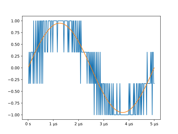
MatPlotLib Example
In this example QuantiPhy is used to create easy to read axis labels in MatPlotLib. It uses NumPy to do a spectral analysis of a signal and then produces an SVG version of the results using MatPlotLib.
#!/usr/bin/env python3

import numpy as np
from numpy.fft import fft, fftfreq, fftshift
import matplotlib as mpl
mpl.use('SVG')
from matplotlib.ticker import FuncFormatter
import matplotlib.pyplot as pl
from quantiphy import Quantity
Quantity.set_prefs(map_sf=Quantity.map_sf_to_sci_notation)

# read the data from delta-sigma.smpl
data = np.fromfile('delta-sigma.smpl', sep=' ')
time, wave = data.reshape((2, len(data)//2), order='F')

# print out basic information about the data
timestep = Quantity(time[1] - time[0], name='Time step', units='s')
nonperiodicity = Quantity(wave[-1] - wave[0], name='Nonperiodicity', units='V')
points = Quantity(len(time), name='Time points')
period = Quantity(timestep * len(time), name='Period', units='s')
freq_res = Quantity(1/period, name='Frequency resolution', units='Hz')
with Quantity.prefs(show_label=True, prec=2):
    print(timestep, nonperiodicity, points, period, freq_res, sep='\n')

# create the window
window = np.kaiser(len(time), 11)/0.37
    # beta=11 corresponds to alpha=3.5 (beta = pi*alpha)
    # the processing gain with alpha=3.5 is 0.37
windowed = window*wave

# transform the data into the frequency domain
spectrum = 2*fftshift(fft(windowed))/len(time)
freq = fftshift(fftfreq(len(wave), timestep))

# define the axis formatting routines
freq_formatter = FuncFormatter(lambda v, p: str(Quantity(v, 'Hz')))
volt_formatter = FuncFormatter(lambda v, p: str(Quantity(v, 'V')))

# generate graphs of the resulting spectrum
fig = pl.figure()
ax = fig.add_subplot(111)
ax.plot(freq, np.absolute(spectrum))
ax.set_yscale('log')
ax.xaxis.set_major_formatter(freq_formatter)
ax.yaxis.set_major_formatter(volt_formatter)
pl.savefig('spectrum.svg')
ax.set_xlim((0, 1e6))
ax.set_ylim((1e-7, 1))
pl.savefig('spectrum-zoomed.svg')
This script produces the following textual output:
Time step = 20 ns
Nonperiodicity = 2.3 pV
Time points = 28k
Period = 560 µs
Frequency resolution = 1.79 kHz
And the following is one of the two graphs produced:
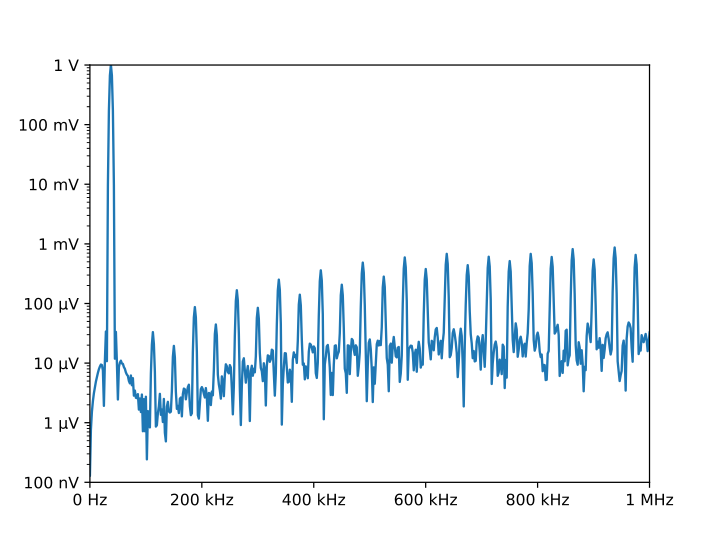
Notice the axis labels in the generated graph. Use of QuantiPhy makes the widely scaled units compact and easy to read.
MatPlotLib provides the EngFormatter that you can use as an alternative to QuantiPhy for formatting your axes with SI scale factors, which also provides the format_eng function for converting floats to strings formatted with SI scale factors and units. So if your needs are limited, as they are in this example, that is generally a good way to go. One aspect of QuantiPhy that you might prefer is the way it handles very large or very small numbers. As the numbers get either very large or very small EngFormatter starts by using unfamiliar scale factors (YZPEzy) and then reverts to e-notation. QuantiPhy allows you to control whether to use unfamiliar scale factors but does not use them by default. It also can be configured to revert to engineering scientific notation (ex: 13.806×10⁻²⁴ J/K) when no scale factors are appropriate. Though not necessary for this example, that was done above with the line:
Quantity.set_prefs(map_sf=Quantity.map_sf_to_sci_notation)
Flicker Noise
This example represents a very typical use of QuantiPhy in a simulation script. As in the two previous examples, it includes both extraction of simulation parameters from the script’s documentation and attractive formatting of units in MatPlotLib graphs. It is a bit long and you cannot run it yourself as it requires access to a proprietary circuit simulator, and as such the code is not included here. But it is an excellent example of how to use QuantiPhy in a variety of ways. You can find the Flicker Noise code on GitHub. It produces results like the following:

Cryptocurrency Example
This example displays the current price of various cryptocurrencies and the total value of a hypothetical portfolio of currencies. QuantiPhy performs conversions from the prices of various currencies to dollars. The latest prices are downloaded from cryptocompare.com. A summary of the prices is printed and then they are multiplied by the portfolio holdings to find the total worth of the portfolio, which is also printed.
It demonstrates some of the features of UnitConversion.
#!/usr/bin/env python3

import requests
from inform import display, fatal, os_error, terminate
from quantiphy import Quantity, UnitConversion, InvalidNumber
Quantity.set_prefs(prec=2)

# read holdings
try:
    with open('holdings') as f:
        lines = f.read().splitlines()
    holdings = {
        q.units: q for q in [
            Quantity(l, ignore_sf=True) for l in lines if l
        ]
    }
except OSError as e:
    fatal(os_error(e))
except InvalidNumber as e:
    fatal(e)

# download latest asset prices from cryptocompare.com
currencies = dict(
    fsyms = ','.join(holdings.keys()),  # from symbols
    tsyms = 'USD',                      # to symbols
)
url_args = '&'.join(f'{k}={v}' for k, v in currencies.items())
base_url = f'https://min-api.cryptocompare.com/data/pricemulti'
url = '?'.join([base_url, url_args])
try:
    response = requests.get(url)
except KeyboardInterrupt:
    terminate('Killed by user.)
except Exception as e:
    fatal('cannot connect to cryptocompare.com.')
conversions = response.json()

# define unit conversions
converters = {
    sym: UnitConversion(('$', 'USD'), sym, conversions[sym]['USD'])
    for sym in holdings
}

# sum total holdings
total = Quantity(sum(q.scale('$') for q in holdings.values()), '$')

# show summary of holdings and conversions
for sym, q in holdings.items():
    value = f'{q:>9q} = {q:<7q$} {100*q.scale("$")/total:.0f}%'
    price = f'1 {sym} = {converters[sym].convert()}'
    display(f'{value:<25s} ({price})')
display(f'    Total = {total:q}')
This script reads a file ‘holdings’ that contains the number of tokens you hold of each of your cryptocurrencies. That file would contain one currency per line and look like this:
10 BTC
100 ETH
100 BCH
100 ZEC
10,000 EOS
100,000 ADA
The output of the script looks like this:
  10 BTC = $65.8k  30%   (1 BTC = $6.58k)
 100 ETH = $22.4k  10%   (1 ETH = $224)
 100 BCH = $51.5k  24%   (1 BCH = $515)
 100 ZEC = $12.7k  6%    (1 ZEC = $127)
 10 kEOS = $57.6k  26%   (1 EOS = $5.76)
100 kADA = $8.16k  4%    (1 ADA = $81.6m)
   Total = $218k
If you prefer the output in fixed-point format, you can replace the last part of this code with:
# show summary of holdings and conversions
for sym, q in holdings.items():
    value = f'{q:>10.2p} = {q:>#11,.2p$}  {100*q.scale("$")/total:,.0f}%'
    price = f'1 {sym} = {converters[sym].convert():>#9,.2p}'
    display(f'{value:<30s} ({price})')
display(f'     Total = {total:>#11,.2p}')
If you do, the output of the script looks like this:
    10 BTC =  $65,847.10  30%  (1 BTC = $6,584.71)
   100 ETH =  $22,401.00  10%  (1 ETH =   $224.01)
   100 BCH =  $51,450.00  24%  (1 BCH =   $514.50)
   100 ZEC =  $12,726.00  6%   (1 ZEC =   $127.26)
 10000 EOS =  $57,600.00  26%  (1 EOS =     $5.76)
100000 ADA =   $8,203.00  4%   (1 ADA =     $0.08)
     Total = $218,227.10
A more sophisticated version of cryptocurrency this example can be found on GitHub.
Dynamic Unit Conversions
Normally unit conversions are static, meaning that once the conversion values are set they do not change during the life of the process. However, that need not be true if functions are used to perform the conversion. In the following example, the current price of Bitcoin is queried from a price service and used in the conversion. The price service is queried each time a conversion is performed, so it is always up-to-date, no matter how long the program runs.
#!/usr/bin/env python3

# Bitcoin
# This example demonstrates how to use UnitConversion to convert between
# bitcoin and dollars at the current price.

from quantiphy import Quantity, UnitConversion
import requests

# get the current bitcoin price from coingecko.com
url = 'https://api.coingecko.com/api/v3/simple/price'
params = dict(ids='bitcoin', vs_currencies='usd')
def get_btc_price():
    try:
        resp = requests.get(url=url, params=params)
        prices = resp.json()
        return prices['bitcoin']['usd']
    except Exception as e:
        print('error: cannot connect to coingecko.com.')

# use UnitConversion from QuantiPhy to perform the conversion
bitcoin_units = ['BTC', 'btc', 'Ƀ', '₿']
satoshi_units = ['sat', 'sats', 'ș']
dollar_units = ['USD', 'usd', '$']
UnitConversion(
    dollar_units, bitcoin_units,
    lambda b: b*get_btc_price(), lambda d: d/get_btc_price()
)
UnitConversion(satoshi_units, bitcoin_units, 1e8)
UnitConversion(
    dollar_units, satoshi_units,
    lambda s: s*get_btc_price()/1e8, lambda d: d/(get_btc_price()/1e8),
)

unit_btc = Quantity('1 BTC')
unit_dollar = Quantity('$1')

print(f'{unit_btc:>8,.2p} = {unit_btc:,.2p$}')
print(f'{unit_dollar:>8,.2p} = {unit_dollar:,.0psat}')
When run, the script prints something like this:
1 BTC = $17,211.91
   $1 = 5,810 sat
Pluralize
Using some external packages you can monkey patch a new method into Quantity that converts quantities into the singular or plural forms of speech.
>>> from quantiphy import Quantity
>>> from inform import plural

>>> def pluralize(self):
...     with self.prefs(form='fixed', show_units=False):
...         return plural(self).format(self.plural_format)

>>> class Loaves(Quantity):
...     units = 'loaves'
...     plural_format = "# /loaf/loaves"
...     pluralize = pluralize

>>> with Quantity.prefs(form='fixed'):
...     for count in [0, 1, 2, 0.5]:
...         q = Loaves(count)
...         print(q, '->', q.pluralize())
0 loaves -> 0 loaves
1 loaves -> 1 loaf
2 loaves -> 2 loaves
0.5 loaves -> 0.5 loaves